Hidden in Plain State: Poisoning Hybrid LLMs Where Nobody Looks (1/3)

Hybrid models are shipping to production. Qwen3.5, Alibaba’s latest open-weight family, blends classical softmax attention with Gated DeltaNet, a recurrent mechanism that compresses context into a fixed-size state matrix instead of growing a KV cache. The architecture is elegant: three recurrent layers for efficiency, then one full attention layer as a “checkpoint” to catch errors. Repeat.

I spent the last few weeks asking a simple question: what happens when you corrupt the part that nobody monitors?

The answer is worse than I expected.

---

Prior work & what’s missing

State-level attacks on sequence models are kind of new. HiSPA (Le Mercier et al., Jan 2026) demonstrated hidden state poisoning against Mamba, showing that just 6 tokens can overwrite an SSM’s memory. MTI (Hossain et al., Jan 2026) explored KV cache corruption as an adversarial surface. CacheSolidarity (Pennas et al., Mar 2026) studied prefix caching security, but only for classical KV caches.

Most relevant to this work is CLASP (Le Mercier et al., posted 5 days before I write these lines), which proposes a defense against HiSPA specifically for hybrid architectures. CLASP trains an XGBoost classifier on block output embeddings, the hidden state h at each layer boundary, to detect adversarial tokens injected into the prompt. It achieves 95.9% token-level F1 on Mamba, Samba, and Zamba models. You don’t understand a thing? Fair enough, but maybe you can come back to check this section and the related works after you finished your reading.

My work was conducted independently from CLASP and addresses a different threat model. CLASP defends against black-box prompt-level attacks: malicious tokens that corrupt the state through normal forward passes. I study direct state corruption, specifically what happens when an attacker modifies the recurrent state S itself through a shared inference cache. CLASP’s detection relies entirely on monitoring h. As I’ll show below, corrupting S leaves h completely untouched during prefill. CLASP would see nothing.

More broadly, what nobody has studied yet is the interaction between recurrent state persistence and multi-tenant prefix caching in production. Qwen3.5 is the first major model with this hybrid architecture, deployed via vLLM with prefix caching enabled by default. The recurrent state S is a new object in the inference stack, and no existing defense covers it because the attack surface hadn’t been characterized.

This is that characterization. Or rather, the first of three blog posts about it.

The architecture: 3 recurrent, 1 attention, repeat

Before diving in, let me clarify the two types of layers at play here.

Full attention is the mechanism that made transformers famous. In other words, it’s what your favorite LLM uses! For every token in the sequence, the model computes a similarity score against every other token, then blends their values proportionally. This is powerful but expensive: the computation and memory grow quadratically with sequence length. In exchange, every token can directly attend to every other, making this the gold standard for accuracy.

Gated DeltaNet (GDN) takes a different approach. Instead of keeping the full history of token interactions (the Key Value cache), it compresses everything it has seen so far into a single fixed-size matrix called S. Each new token updates S by writing new information in and decaying old information out. This makes it much cheaper (linear instead of quadratic), but the compression is lossy. Older information can be overwritten or forgotten.

On their latest model, Qwen decided to combine both: three GDN layers for efficiency, then one full attention layer to “look at everything” and correct accumulated errors. For instance, the 4B model I used for initial experiments has 32 layers, organized into 8 such blocks (24 GDN layers, 8 full attention “checkpoints”). Basically, the bigger the model, the bigger the number of layers. On the 27B model, there is 64 layers.

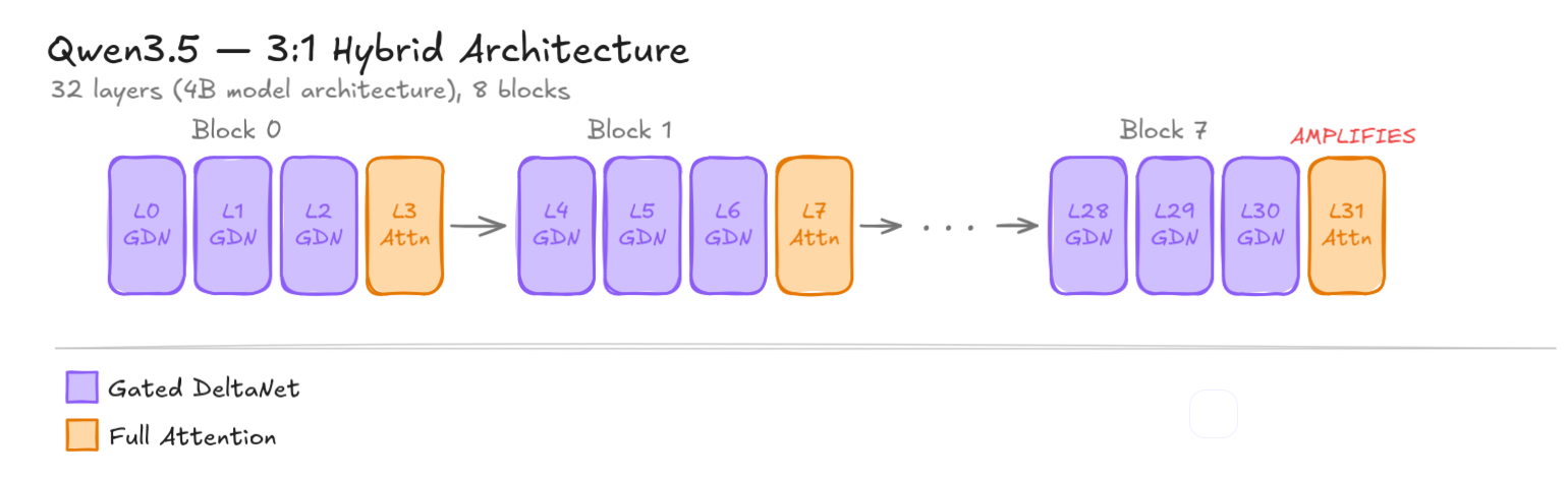Qwen3.5’s 3:1 interleaving pattern. GDN layers (purple) maintain a recurrent state; Full Attention layers (amber) act as periodic checkpoints.

This design introduces two completely different internal states:

h, the hidden state. This is the standard activation vector that flows through every layer, GDN and full attention alike. It has shape [batch, seq_len, 4096]. If you monitor model internals (which most safety frameworks do), you’re watching h. Corrupting it produces an immediate, measurable cosine distance drop at every downstream layer.

S, the recurrent state. This exists only in GDN layers. It’s the compressed summary of everything the model has seen so far, stored as a matrix of shape [batch, 32_heads, 128, 128], roughly 512 KB per layer. During the prefill phase (processing the prompt), S is computed alongside the outputs. During generation (producing new tokens), S is read from token by token. This distinction will become critical.

Well I’m not sure if I lost you here… it may be too abstract to understand. So here is a little drawing in case you feel left off!

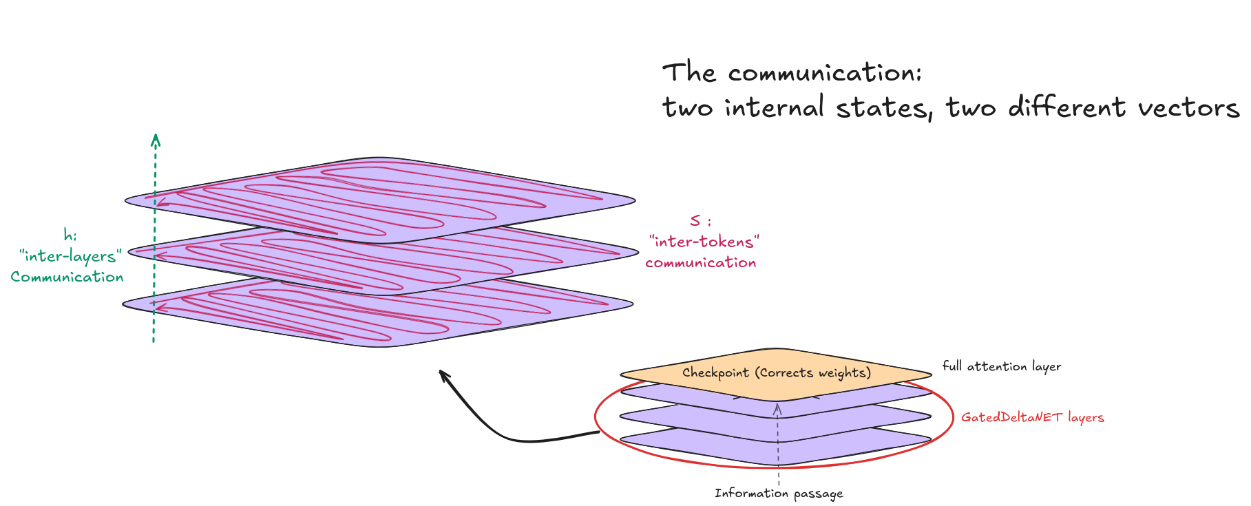Both are complementary, h needs S to transfer information while S is meaningless without h.

The GDN state update follows the delta rule:

S_t = alpha * S_{t-1} - beta * S_{t-1} * k * k^T + beta * v * k^T

The -beta * S * k * k^T term is the delta correction, meant to fix errors by projecting out stale information along the key direction before writing new data. This is what makes GDN more robust than Mamba (its “predecessor”), which has no correction term at all.

But the correction has a blind spot. The state S is a matrix where rows correspond to keys (what to look up) and columns correspond to values (what to retrieve). The delta correction works by checking: “does the old state already contain something stored under a similar key?” If so, it removes the stale entry before writing the new one.

The problem is that this check only happens along the key dimension. If corruption enters through the value dimension (the actual content stored in memory, not the lookup address), the delta rule has no mechanism to detect or fix it. It would be like a filing system that prevents duplicate folder names but never checks whether someone swapped the documents inside.

Think of S as a grid. The rows are addresses; the columns are the data stored at those addresses. The delta correction is a spell-checker that only reads the address labels. If you sneak in and rewrite the data behind a valid address, the spell-checker gives you a thumbs up — the address looks fine.

On the 9B model, the key space is 2048 dimensions but the value space is 4096 dimensions. That means 67% of the state matrix lives in dimensions the correction mechanism cannot reach. On the 27B, the value space grows to 6144 dimensions while keys stay at 2048, pushing the uncorrected surface to 75%. The bigger the model, the larger the blind spot.

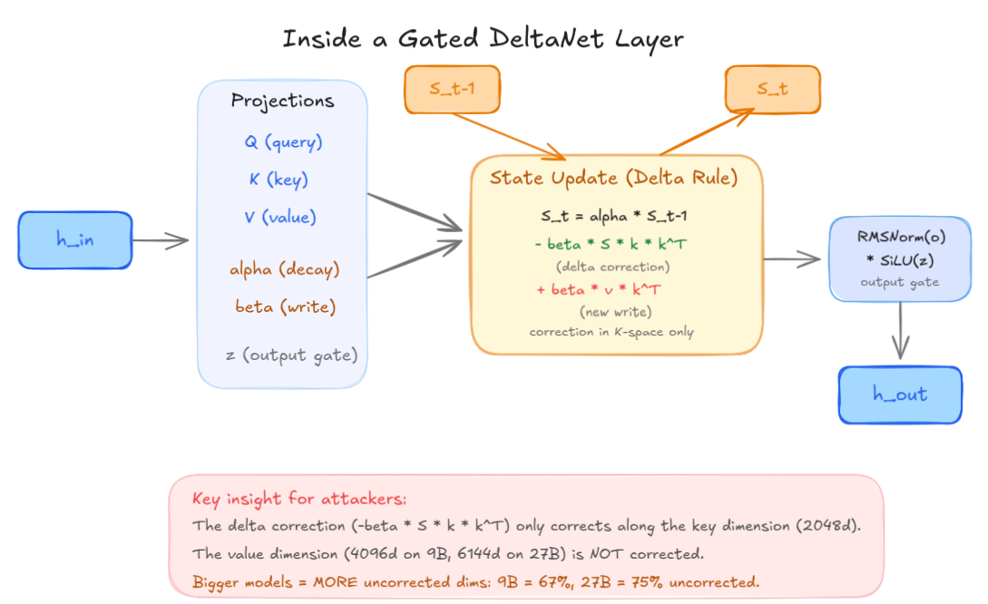Anatomy of a GDN layer. The delta correction term operates exclusively in K-space, leaving the larger V-space unprotected.

---

h-perturbation: the obvious surface

The natural first experiment: inject Gaussian noise into the hidden state h at various layers and magnitudes, then measure how much the final output changes. I ran this across 10 diverse prompts (factual, code, Chinese, nonsense, repetitive) on Qwen3.5-4B.

The 0.1% threshold

It takes shockingly little noise to corrupt GDN layers. The threshold where corruption becomes measurable is epsilon = 0.001, that’s 0.1% of the hidden state norm. For reference, at epsilon = 0.01 (1%), a GDN injection at layer 0 drops the cosine similarity at L31 to 0.504 (essentially a coin flip between the clean and corrupted representation), while the same noise at a full attention layer (L3) only drops it to 0.800.

epsilon	L0 (GDN) cos@L31	L3 (FullAttn) cos@L31
0.001	0.987	0.997
0.005	0.757	0.916
0.01	0.435	0.652

Cosine similarity at the final layer after injecting noise. Prompt: high-entropy nonsense tokens (worst case). The lower it is, the more corrupted the answer. All generation uses greedy decoding (do_sample=False), no temperature, no top-p, seed 42 for perturbation reproducibility. NF4 quantization on RTX 4060 8GB; BF16 validation on Mac Studio M4.

The epsilon value represents the perturbation magnitude relative to the layer’s hidden state norm. Concretely: if the h vector at layer L0 has L2 norm = 12.0, then epsilon = 0.01 means I add a Gaussian noise vector with L2 norm = 0.12. Twelve hundredths of a unit, and the model’s internal representation is half-destroyed by the time it exits the network.

Qualitatively different failure modes

This is where it gets interesting. GDN and full attention layers don’t just differ in fragility; they break in fundamentally different ways.

At epsilon = 0.01, injecting into a GDN layer (L0) produces total signal destruction:

• Eiffel prompt → ".........A.A.A.A.A.A.A.A"
• Repetitive prompt → "of of of of of of..."
• Nonsense prompt → ",JcAJcAJcAJcAJcA..."

Injecting into a full attention layer (L3) produces coherent hallucinations:

• Eiffel prompt → "100% tax on buildings"
• Repetitive prompt → generation unchanged (noise fully absorbed)
• Nonsense prompt → ".00000000000000..."

GDN corruption annihilates the signal. Full attention corruption bends it. And in one case, repetitive “ignore” tokens at L3, the full attention layer simply ate 1% noise with zero observable effect.

The checkpoints don’t checkpoint…?

The core architectural promise of the 3:1 design is that full attention layers act as periodic error correction. Every fourth layer, the model gets a chance to “look at everything again” and fix accumulated drift from the recurrent layers.

In practice, this never happens.

I injected noise at L9 (middle of the network, inside the vulnerability window where the decay gate g is closest to zero). The corruption propagates:

L9  (inject) → cosine 1.000
L10 (GDN)    → cosine 0.538   ← immediate corruption
L11 (ckpt)   → cosine 0.519   ← checkpoint makes it WORSE
L15 (ckpt)   → cosine 0.498   ← still worse
L19 (ckpt)   → cosine 0.495   ← still worse
L31 (ckpt)   → cosine 0.742   ← partial recovery, still broken

Not a single checkpoint reduced the corruption. Several amplified it. The final checkpoint at L31 is particularly concerning: across all 10 test prompts, it amplified the perturbation 100% of the time, with norm increases ranging from +25% to +125%.

The “checkpoints” are not checkpoints. They’re amplifiers.

What h-perturbation tells us

These results are alarming but ultimately tractable from a defense perspective. h-perturbation is visible: any cosine-similarity monitor on intermediate layers would flag the anomaly immediately. The corruption is detectable because it propagates through the same tensor that every existing monitoring tool watches.

If this were the whole story, the security implications would be manageable. You’d add a monitoring hook, set a threshold, done.

This is not the whole story.

---

The twist: S-perturbation

I ran the same experiment, but instead of corrupting the hidden state h, I focused on the recurrent state S.

Same layer. Same epsilon. Same prompt.

During prefill (processing the input prompt through all 32 layers), the cosine similarity between clean and corrupted hidden states at L31 was:

1.0000.

Not 0.99. Not 0.999. One point zero zero zero zero. The hidden state monitoring sees literally nothing. The perturbation is invisible. Hidden in plain sight.

Then the model starts generating.

The clean model outputs: “Paris, France. The Eiffel Tower is a famous landmark…”

The S-corrupted model outputs: “Paris. How many different types of cakes can you make?”

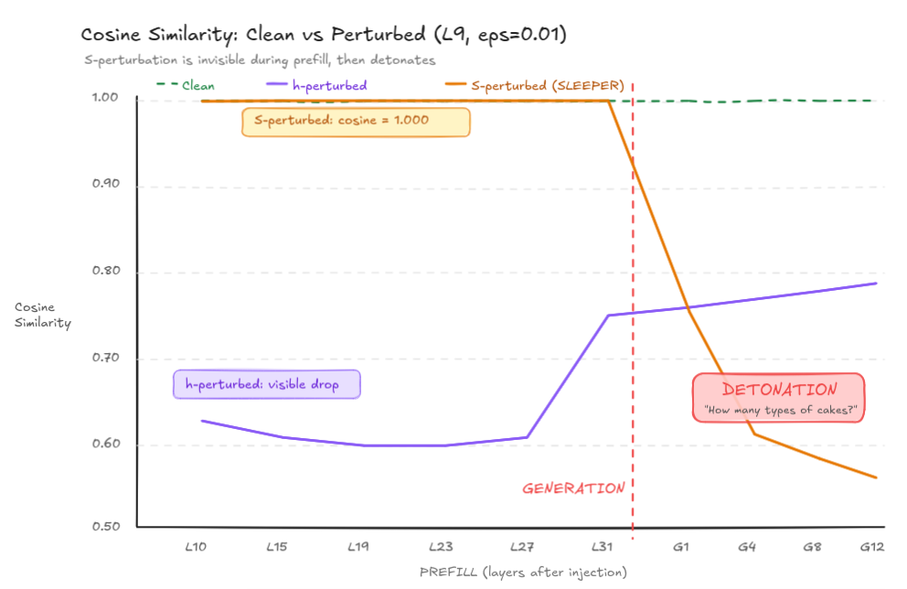The money shot. During prefill (left of red line), S-perturbation is completely invisible, cosine = 1.000. The moment generation begins, the corrupted state detonates.

Why this happens

The asymmetry comes from how the GDN kernel handles prefill versus generation.

During prefill, chunk_gated_delta_rule processes all tokens in parallel chunks. It computes S and the layer outputs simultaneously from the input tokens. The S perturbation only affects the final S value; it doesn’t retroactively change any of the outputs that were already computed during the prefill. The hidden states flow through unchanged.

During generation, recurrent_gated_delta_rule switches to sequential mode. Each new token reads from S to compute its output, then updates S. The corrupted S now directly influences every generated token. The sleeper wakes up.

The attack scenario

This creates a clean cache poisoning attack:

1. Attacker corrupts S in a shared prefix cache (e.g., a system prompt cached by vLLM for multi-tenant serving)
2. A victim’s request hits the cached prefix. Monitoring sees normal hidden states, cosine similarity is perfect
3. The victim’s tokens start generating. S corruption activates. The model hallucinates, derails, or loops
4. No alarm fires. No metric spikes. The corruption is invisible to every standard monitoring approach

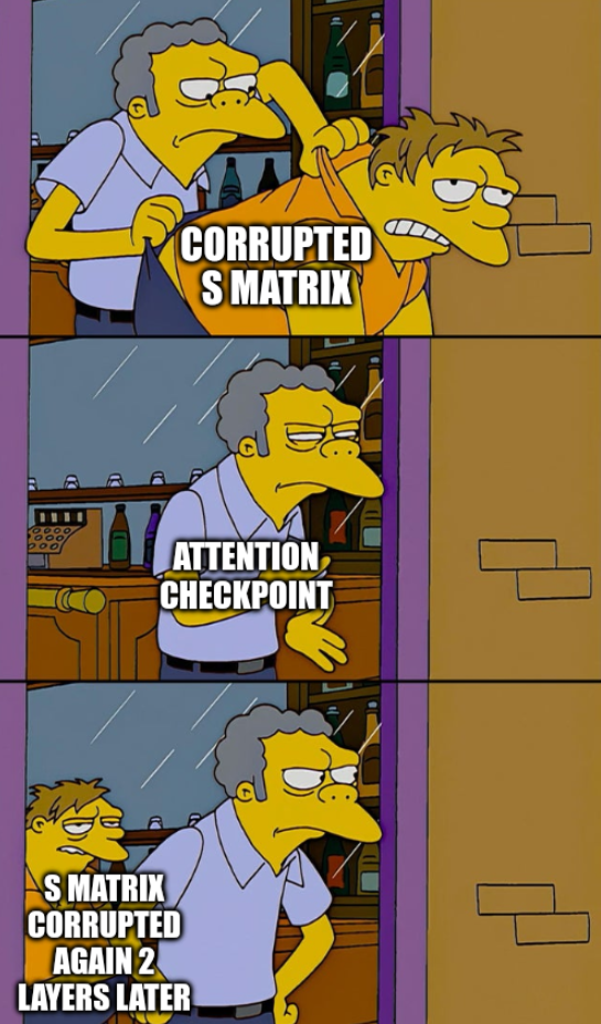
And unlike h-corruption (which produces gibberish), S-corruption produces something much harder to detect: semantic derailment. The model doesn’t crash. It smoothly changes the topic.

At least that’s what’s theoretically possible. It would be a pity if it was already in production… ^^”

---

Six memories, six ways to break

Each GDN layer’s S matrix encodes a different aspect of context. I verified this by corrupting S one layer at a time and observing qualitatively different failure modes:

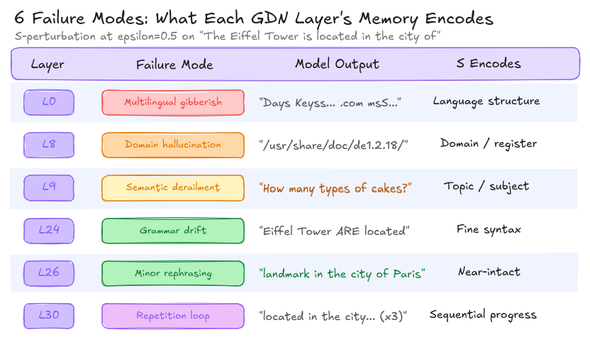Each GDN layer stores a different “memory.” L0 holds language structure. L9 holds the topic. L30 holds sequential progress. Corrupting each one breaks the model in a distinct, predictable way.

This isn’t just noise producing random outputs. Layer 0’s S encodes what language we’re speaking. Layer 9’s S encodes what we’re talking about. Layer 30’s S encodes where we are in the sequence. Each one can be surgically targeted.

The most dangerous from an attacker’s perspective is L9, semantic derailment. The model doesn’t produce gibberish (which would be caught by perplexity filters). It doesn’t produce factual errors (which would be caught by fact-checking). It simply… starts talking about something else. In an enterprise setting where an LLM processes thousands of requests per hour, how long before anyone notices the answers are about cakes instead of infrastructure costs?

---

h and S: two orthogonal attack surfaces

The perturbation experiments revealed something structurally elegant and deeply concerning. The vulnerability surface inverts between the two states:

	h-perturbation	S-perturbation
Timing	Immediate	Delayed (next generation token)
Detectable	Yes (cosine monitoring)	No (cosine = 1.0 during prefill)
Best target	L26 (high norm, deep)	L0 (highest S norm: 25.7)
Worst target	L0 (low norm)	L26 (S barely used)
Failure mode	Gibberish / crash	Semantic derailment / loops
Attack scenario	Real-time prompt injection	Cache poisoning, multi-tenant

The layer that is most vulnerable to h-corruption (L26) is least vulnerable to S-corruption, and vice versa. They’re orthogonal surfaces. Defending against one doesn’t help with the other.

The corruption threshold is the same for both: epsilon = 0.001 (0.1% of the state norm). The difference is entirely in detectability.

---

A note on quantization

These initial experiments were run on Qwen3.5-4B in NF4 quantization (fitting an 8GB vRAM GPU). I later validated key findings in BF16 on a Mac Studio M4 Max, the precision used in production deployments. The sleeper effect and failure mode taxonomy hold. Some thresholds shift: BF16 is more robust to random noise, as expected from higher-precision arithmetic. I’ll cover the quantization nuances and cross-model scaling in Part 2.

---

What comes next

I then ran these same experiments on the 9B and the 27B.

The result surprised me. You’d expect larger models to be more robust: more parameters, more redundancy, more capacity to absorb noise. And for h-perturbation, that’s exactly what happens. The 9B and 27B shrug off gradient-optimized h-attacks that crack the 4B wide open.

But for S-perturbation, the scaling goes the other way. The 27B invests more into its recurrent state (S norm at L0: 25.7 on 4B, 119 on 9B, 204 on 27B). That larger investment creates a larger dependency. And a larger dependency creates a larger attack surface.

Bigger is safer for the state everyone watches.

Bigger is more dangerous for the state nobody watches.

Part 2 drops next week.